How to Optimize a Battery in ERCOT (pre-RTC+B)
Introduction
Grid-scale batteries can profit by buying electricity when prices are low and selling when prices spike. In ERCOT’s 5-minute real-time market, prices can swing from near-zero to hundreds of dollars per MWh within hours—creating significant arbitrage opportunities, like they did at Rabit Hill (RHESS2_ESS1) back in February 2025.
With that in mind, I built esrpy, a Python library for backtesting battery optimization and trading strategies for RT energy arbitrage in ERCOT. This post describes how the optimization works and what I learned about how the strategy would do on actual data.
The Optimization Problem
The core strategy uses cvxpy to solve a linear program at each 5-minute interval, looking 55 minutes ahead (11 intervals). The objective is simple: maximize revenue.
maximize Σ(t=0 to 10) [power[t] × price[t] × Δt]Subject to physical constraints:
- SoC limits: Battery can’t go below minimum or above maximum capacity
- Power limits: Charge/discharge rate capped at rated power
- Energy conservation:
soc[t+1] = soc[t] - power[t] × Δt / η
After solving, the strategy applies post-processing to avoid trading in unfavorable conditions—a practical “bandaid” for not explicitly modeling cycling costs in the objective.
Running a Backtest
Using esrpy with the appropriate set of input data (see here), one can run a backtest like this.
from esrpy import (
    BacktestConfig,
    BatteryConfig,
    ConfigurableOptimizationStrategy,
    PointInTimeData,
    load_lmps,
    run_backtest,
)

forecast_lmps, actual_lmps = load_lmps(
    actual_csv_path="actual_lmps.csv",
    forecast_csv_path="forecast_lmps.csv",
)

pit_data = PointInTimeData(forecast_lmps, actual_lmps)

results_df = run_backtest(
    pit_data=pit_data,
    strategy=ConfigurableOptimizationStrategy(),
    battery_config=BatteryConfig(),
    backtest_config=BacktestConfig(),
)
Results: One Week in October 2025
I compared three strategies on a simulated 100 MW / 100 MWh battery, using real ERCOT data for Oct. 1-7, 2025, at the RHESS2_ESS1 node. (5-minute indicative prices were used for forecasts.)
| Strategy | Total PnL | Cycles |
|---|---|---|
| Simple threshold | $17,511 | 2.8 |
| Battery optimization | $18,430 | 5.9 |
| Perfect foresight | $31,540 | 10.4 |
Simple Threshold: Leaving Money on the Table
The simple threshold strategy uses naive rules: sell if forecasted price > $100, buy if forecasted price < $10. While it generated positive returns, the extremely low cycling (2.77 cycles) reveals a fundamental issue—the thresholds were too conservative. This cautious trading behavior left profitable opportunities on the table, resulting in the lowest PnL of the three strategies.
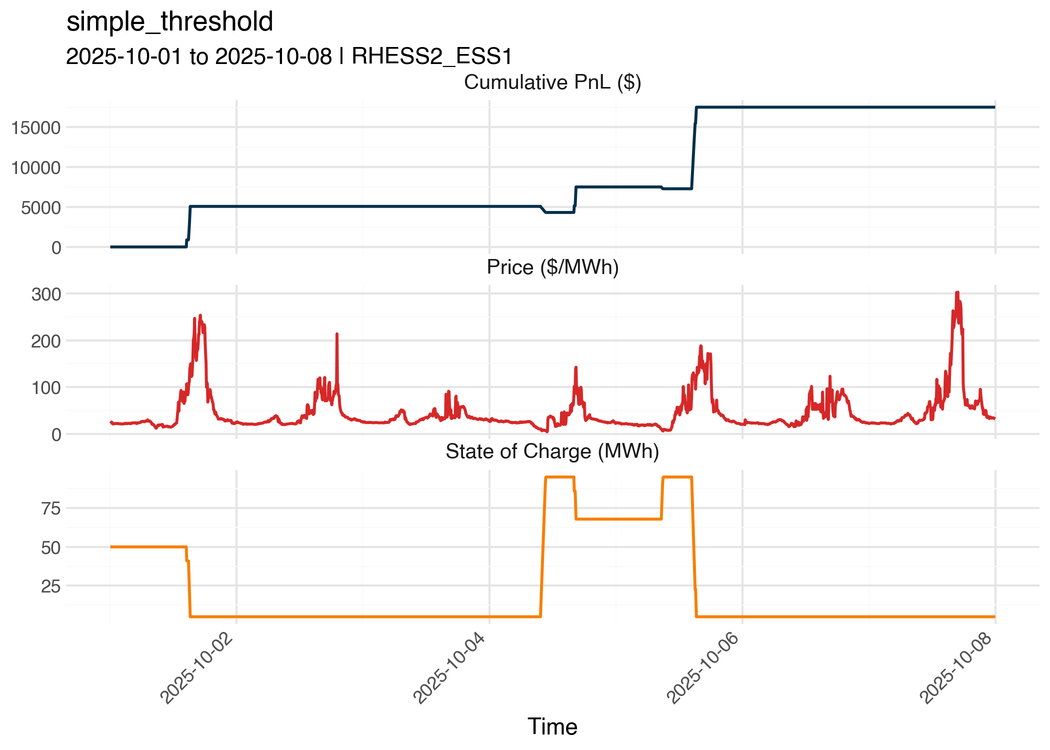
The gap between this approach and battery optimization suggests that even modest sophistication in strategy design can capture meaningful additional value.
Battery Optimization: Balancing Returns and Cycling
The LP-based optimization strategy achieved a respectable ~$18.4K PnL with moderate cycling (~6 cycles), striking a reasonable balance between capturing spreads and managing battery wear. This 5% improvement over simple thresholds demonstrates the value of dynamic optimization.
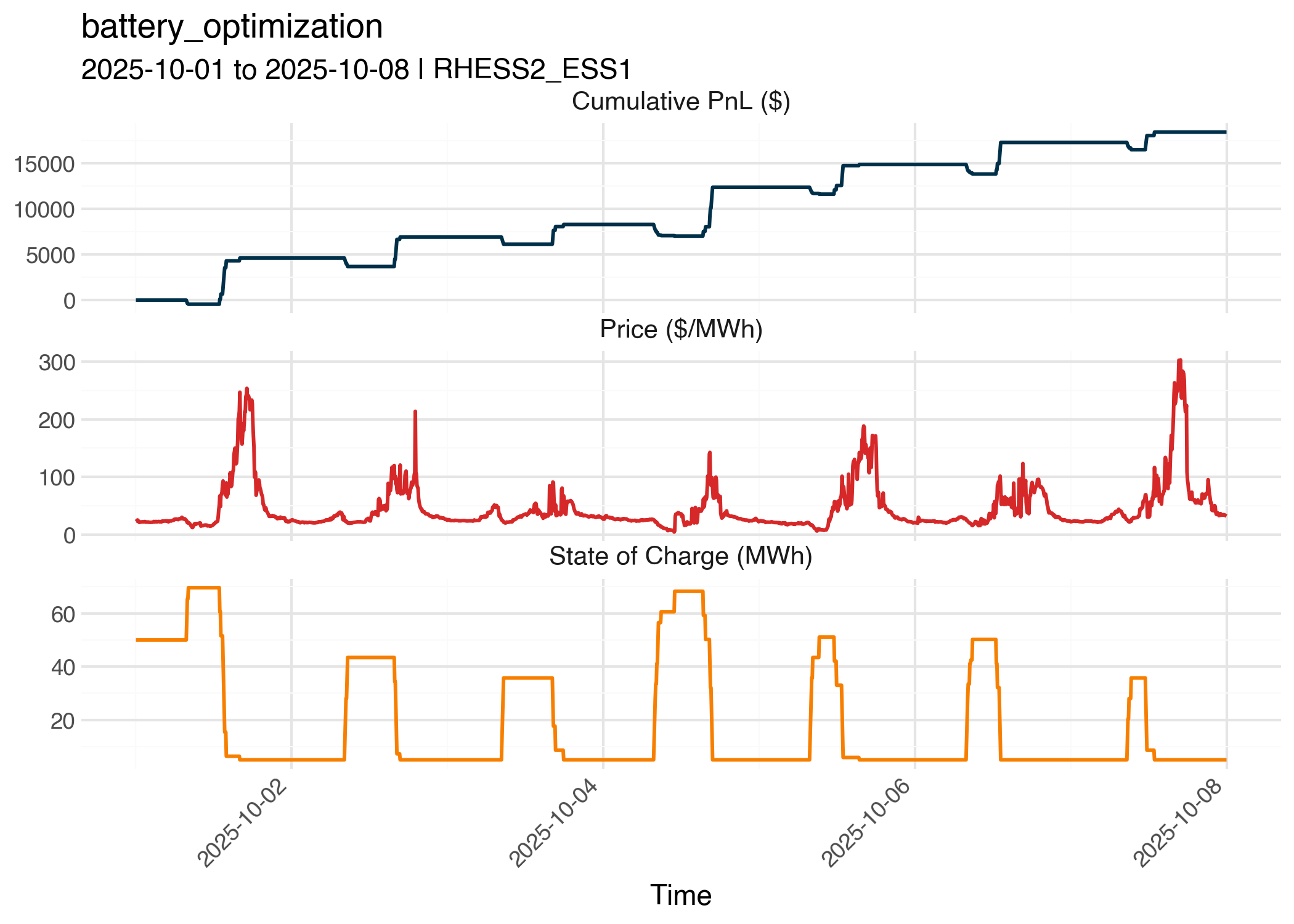
However, there’s a key limitation: the optimizer only sees 11 intervals (~55 minutes) ahead. This short horizon may cause it to miss longer-term price patterns and manage state-of-charge suboptimally. For instance, if a major price spike is forecasted 3 hours out, the battery might discharge too early on smaller spreads, leaving insufficient capacity for the larger opportunity.
A longer forecast horizon—perhaps 12 hours—could help the optimizer anticipate these larger price swings and make more strategic decisions about when to preserve capacity.
Perfect Foresight: The Value of Better Forecasting
The perfect foresight strategy sets the theoretical upper bound, achieving ~$31.5K by knowing future prices exactly and aggressively trading around price spreads. The ~$13K gap between perfect foresight and battery optimization represents the theoretical value of improved forecasting for the LP approach.
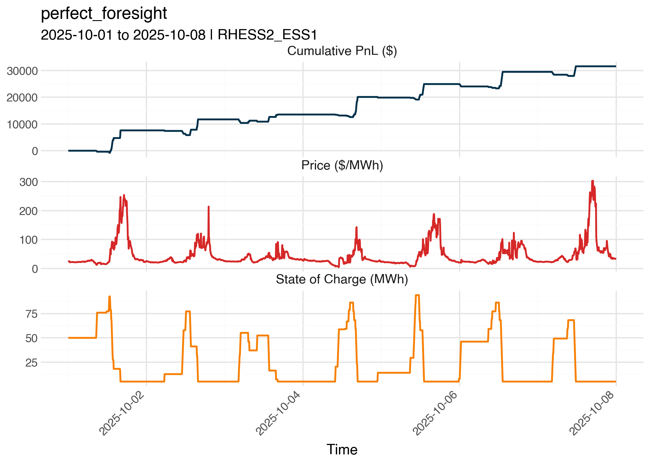
But there’s an important caveat: perfect foresight cycled nearly twice as much as battery optimization (~10 vs ~6 cycles). This aggressive cycling would face penalties if hurdle costs or degradation were properly modeled in the objective function. In practice, the PnL advantage would shrink once you account for the real cost of battery wear from those extra cycles.
Key Takeaways
- Even simple optimization beats naive thresholds — the LP approach earned 5% more PnL
- Forecast horizon matters — 55 minutes may miss larger daily patterns
- Perfect foresight reveals two things: the upside of better forecasting (~$13K) and the importance of modeling cycling costs (nearly 2x cycles vs. battery optimization)
- This is just RT energy — post-RTC+B, the real opportunity (and complexity) lies in co-optimizing across energy and AS products in real-time
Appendix
Scope: Real-time Energy Arbitrage
This work focuses specifically on real-time (RT) energy arbitrage—buying and selling energy in ERCOT’s 5-minute market. It’s worth understanding what this doesn’t cover:
Day-Ahead Market (DAM): Trading in the DAM requires a fundamentally different approach. You’re committing to positions ~24 hours in advance based on forecasts, with settlement against actual RT prices. The optimization horizon extends to 24+ hours, and you’re essentially making bets on DA/RT price spreads. The uncertainty is much higher, and position sizing becomes critical.
Ancillary Services (AS): Historically, AS has been procured entirely in the DAM. If you committed 20 MW to Responsive Reserve Service (RRS), those megawatts were locked up and unavailable for RT energy arbitrage.
What changes with RTC+B: On December 5, 2025, ERCOT implements Real-Time Co-Optimization plus Batteries (RTC+B). This fundamentally changes the game:
- AS will be co-optimized with energy in real-time, not just cleared day-ahead
- SCED will see your full battery capability every 5 minutes and decide whether energy or AS is more valuable
- DAM commitments become purely financial—you can adjust your RT strategy based on actual conditions
- Storage assets get up to 10 bid pairs per interval for energy and 5 for AS
The optimization problem becomes much more complex under RTC+B. You’d need to co-optimize across energy and multiple AS products (Reg Up, Reg Down, RRS, ECRS, Non-Spin) every 5 minutes, weighing opportunity costs, SoC management, and penalty exposure simultaneously.
This code is a good starting point for understanding RT energy optimization in isolation—but would need significant expansion to handle post-RTC+B AS trading.