Basic Usage
basic-usage.Rmd
library(dplyr)
library(magrittr)
library(ffsched)

# Just for plotting
library(ggplot2)
library(forcats)
library(scales)
league_id <- 899513
weeks <- 12
league_size <- 10
season <- 2020
sims <- 1000
tries <- 0.1 * sims
Simulate 1000 unique schedules for a 10-team league for the first 12 weeks. Note that you don’t need the league_id for this!
set.seed(42) # For repoducibility
sched_sims <-
  generate_schedules(
    league_size = league_size,
    sims = sims,
    tries = tries
  )
sched_sims
#> # A tibble: 120,000 x 4
#>    idx_sim  week team_id opponent_id
#>      <int> <dbl>   <int>       <int>
#>  1       1     1       1           2
#>  2       1     1       2           1
#>  3       1     1       3           8
#>  4       1     1       4           5
#>  5       1     1       5           4
#>  6       1     1       6           7
#>  7       1     1       7           6
#>  8       1     1       8           3
#>  9       1     1       9          10
#> 10       1     1      10           9
#> # … with 119,990 more rows
Get fantasy football scores from ESPN.
scores <-
  scrape_espn_ff_scores(
    league_id = league_id,
    league_size = league_size,
    season = season,
    weeks = weeks
  )
scores
#> # A tibble: 120 x 14
#>    team_id opponent_id team           week team_home_id team_away_id points_home
#>      <dbl>       <dbl> <chr>         <dbl>        <dbl>        <dbl>       <dbl>
#>  1       1           4 The Early GG…     1            4            1       130.
#>  2       1           5 The Early GG…     2            5            1       163.
#>  3       1           3 The Early GG…     3            3            1       119.
#>  4       1           8 The Early GG…     4            8            1        95.2
#>  5       1           7 The Early GG…     5            7            1       127.
#>  6       1           2 The Early GG…     6            2            1       146.
#>  7       1           6 The Early GG…     7            6            1       101.
#>  8       1          10 The Early GG…     8           10            1       152.
#>  9       1           9 The Early GG…     9            9            1       138.
#> 10       1           5 The Early GG…    10            5            1       162.
#> # … with 110 more rows, and 7 more variables: points_away <dbl>,
#> #   team_home <chr>, team_away <chr>, team_winner_id <dbl>, pf <dbl>, pa <dbl>,
#> #   is_winner <lgl>
Join the simulated schedules and the actual scores together to come up with simulated standings.
anonymize_teams <- function(data) {
  data %>%
    mutate(
      across(team, ~sprintf('Team %02d', team_id))
    )
}
scores_by_team <- scores %>% select(team_id, team, week, pf)

scores_sims <-
  sched_sims %>%
  left_join(
    scores_by_team,
    by = c('week', 'team_id')
  ) %>%
  left_join(
    scores_by_team %>%
      dplyr::rename(opponent_id = .data$team_id, opponent = .data$team, pa = .data$pf),
    by = c('week', 'opponent_id')
  ) %>%
  mutate(
    w = if_else(pf > pa, 1L, 0L)
  )

standings_sims <-
  scores_sims %>%
  group_by(idx_sim, team, team_id) %>%
  summarize(
    across(c(pf, w), sum)
  ) %>%
  ungroup() %>%
  group_by(idx_sim) %>%
  mutate(
    rank_w = min_rank(-w)
  ) %>%
  ungroup() %>%
  group_by(idx_sim, rank_w) %>%
  mutate(
    rank_tiebreak = row_number(-pf) - 1L
  ) %>%
  ungroup() %>%
  mutate(rank = rank_w + rank_tiebreak) %>%
  select(-rank_w, -rank_tiebreak) %>%
  anonymize_teams()
standings_sims
#> # A tibble: 10,000 x 6
#>    idx_sim team    team_id    pf     w  rank
#>      <int> <chr>     <dbl> <dbl> <int> <int>
#>  1       1 Team 10      10 1336.     5     8
#>  2       1 Team 08       8 1480.     6     6
#>  3       1 Team 02       2 1561.     7     4
#>  4       1 Team 04       4 1448.     3     9
#>  5       1 Team 06       6 1609.    10     1
#>  6       1 Team 03       3 1484.     6     5
#>  7       1 Team 09       9 1562.     5     7
#>  8       1 Team 01       1 1313.     2    10
#>  9       1 Team 05       5 1620.     7     3
#> 10       1 Team 07       7 1677.     9     2
#> # … with 9,990 more rows
standings_sims can be achieved by using the do_simulate_standings function, which wraps the functionality demonstrated above.
standings_sims <-
  do_simulate_standings(
    league_id = league_id,
    league_size = league_size,
    season = season,
    weeks = weeks,
    sims = sims,
    tries = tries
  ) %>%
  anonymize_teams()
standings_sims
#> # A tibble: 10,000 x 6
#> idx_sim team team_id pf w rank
#> <int> <chr> <dbl> <dbl> <int> <int>
#> 1 1 Team 10 10 1336. 5 8
#> 2 1 Team 08 8 1480. 6 6
#> 3 1 Team 02 2 1561. 7 4
#> 4 1 Team 04 4 1448. 3 9
#> 5 1 Team 06 6 1609. 10 1
#> 6 1 Team 03 3 1484. 6 5
#> 7 1 Team 09 9 1562. 5 7
#> 8 1 Team 01 1 1313. 2 10
#> 9 1 Team 05 5 1620. 7 3
#> 10 1 Team 07 7 1677. 9 2
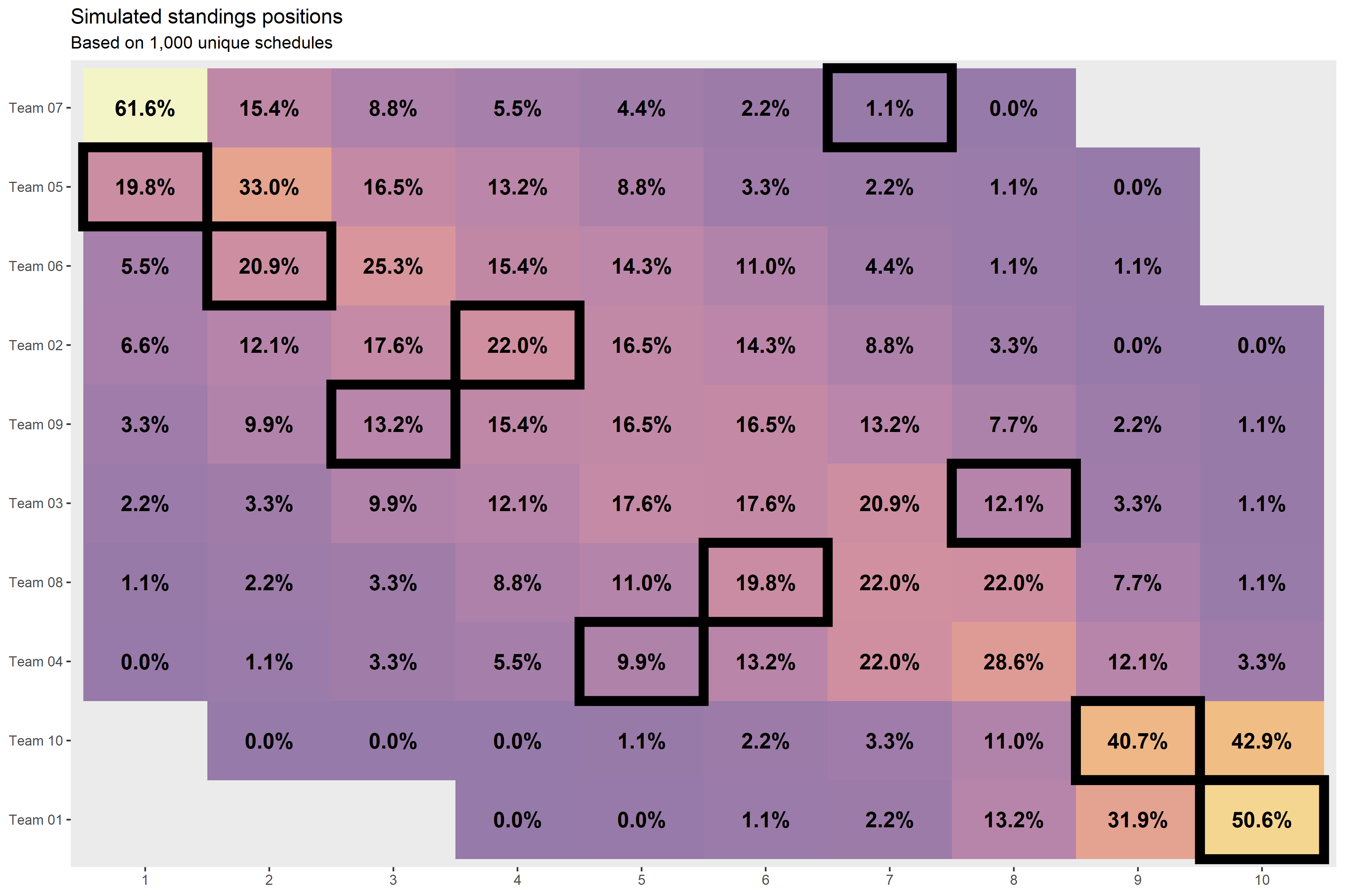
#> # … with 9,990 more rowsMake an interesting plot.
standings_sims_n <-
  standings_sims %>%
  count(team_id, team, rank, sort = TRUE) %>%
  group_by(team_id, team) %>%
  mutate(frac = n / sum(n)) %>%
  ungroup()
standings_sims_n

standings_sims_n_top <-
  standings_sims_n %>%
  group_by(rank) %>%
  slice_max(n, with_ties = FALSE) %>%
  ungroup()
standings_sims_n_top

standings_sims_n_top <-
  standings_sims_n %>%
  group_by(team) %>%
  summarize(
    tot = sum(n),
    rank_avg = sum(rank * n)  / tot
  ) %>%
  ungroup() %>%
  mutate(rank_tot = row_number(rank_avg)) %>%
  arrange(rank_tot)
standings_sims_n_top

standings_actual <-
  scores %>%
  anonymize_teams() %>%
  mutate(w = if_else(pf > pa, 1, 0)) %>%
  group_by(team, team_id) %>%
  summarize(
    across(c(w, pf), sum)
  ) %>%
  ungroup() %>%
  mutate(rank_w = min_rank(-w)) %>%
  group_by(rank_w) %>%
  mutate(
    rank_tiebreak = row_number(-pf) - 1L
  ) %>%
  ungroup() %>%
  mutate(rank = rank_w + rank_tiebreak)
standings_actual

factor_cols <- function(data) {
  data %>%
    left_join(
      standings_sims_n_top %>%
        select(team, rank_tot, rank_avg)
    ) %>%
    left_join(standings_actual) %>%
    mutate(
      across(team, ~fct_reorder(.x, -rank_tot)),
      across(rank, ordered)
    )
}

pts <- function(x) {
  as.numeric(grid::convertUnit(grid::unit(x, 'pt'), 'mm'))
}

viz_standings_tile <-
  standings_sims_n %>%
  factor_cols() %>%
  ggplot() +
  aes(x = rank, y = team) +
  geom_tile(aes(fill = frac), alpha = 0.5, na.rm = FALSE) +
  geom_tile(
    data = standings_actual %>% factor_cols(),
    fill = NA,
    color = 'black',
    size = 3
  ) +
  geom_text(
    aes(label = percent(frac, accuracy = 1.1)),
    color = 'black',
    size = pts(14),
    fontface = 'bold'
  ) +
  scale_fill_viridis_c(option = 'B', begin = 0.2, end = 1) +
  guides(fill = FALSE) +
  theme(
    panel.grid.major = element_blank(),
    panel.grid.minor = element_blank(),
  ) +
  labs(
    title = 'Simulated standings positions',
    subtitle = sprintf('Based on %s unique schedules', comma(sims)),
    x = NULL,
    y = NULL
  )
viz_standings_tile