5 Indifferent Probability and the NBA Draft

The value of NBA draft picks relative to can be calculated using the concept of indifferent probability (IP), a term I briefly referenced in a previous chapter highlighting the value of information in the context of the NBA draft. I believe that IPs can be used to extend my analysis in another chapter covering how to estimate the value of NBA draft picks.

Specifically, we might use them to learn about which picks are most cost-effective and what the trade value of picks is (in terms of other picks). In other words, I can find an answer to the second question “At which draft slots does the expected basketball production outperform the contractual obligation the most?”) that I posed in my review of existing research on the topic of NBA draft pick value, as well as answer to the first question (“What is the relative trade value of picks?”) that I asked in its[follow-up chapter;

However, just as I did in my post discussing the value of perfect information and the NBA draft, let me first provide a quick overview IPs in a theoretical context.

5.1 Indifferent Probability, in Theory

For those of you who are not as familiar with utility theory or decision analysis, IPs are simply relative probabilities that define the degree of preference with respect to (usually) two other outcomes—one more—desirable and one less desirable. IPs are relatively straightforward to calculate. An IP is just the ratio of the difference between a given value and a pre-defined minimum value with the difference of a pre-defined maximum value with the same minimum value. Less formally, it can be written (given value - min value) / (max value - min value). In reality, we can calculate IPs with respect to any two points in a data set as long as the value of interest is not be greater than the maximum value or less than the minimum value.

A better understanding of IPs is perhaps best acquired through an example. To stay within the realm of the sports before considering the application of IPs to NBA draft pick value, let us imagine a typical sports fan who has the autograph of his favorite player on his favorite team. Now, let’s say he has the option to play a dual-outcome game of chance in exchange for giving up his autographed item. If he wins, then he is granted the opportunity to spend an entire day with his favorite player; if he loses, then he receives nothing. Clearly, the first outcome is preferable to the second. Furthermore, the existing state of possessing the autographed item is less preferable to the first and more preferable to the second.

The IP is the likelihood of winning the game (states as a probability) that would make the sports fan feel comfortable with (or, more precisely, indifferent to) giving up his autographed item and playing the game. If we imagine that the fan perceives the first outcome—the opportunity to spend a day with his favorite player—to be only slightly more preferable to the existing state—possessing the autograph—then his IP would be relatively high (e.g. ~0.75 to 1 probability, or ~75% to 100% percent chance). Similarly, the IP would be relatively high if the fan perceives the second outcome—receiving nothing—is significantly less preferable to the existing state.

Intuitively, this should make sense: assuming that the prior two statements are true, then the fan would have to know that there is a high probability of winning the game of chance because he would strongly despise the outcome if he were to lose and only receive a relatively slight bit of enjoyment if he were to win. (Note that a high IP only necessitates that only one of the prior two statements is true, although its numerical value increases even more if both statements are valid.)

5.2 Indifferent Probability for (First-Round) NBA Draft Picks

With this higher-level discussion of IPs out of the way, let’s take another look at our prior our estimates of the cost, value, and profit of first-round NBA draft picks. For reference, in Figure 1 and 2 I have reproduced the empirical and theoretical raw and regressed data sets shown in figures in my chapter on general NBA draft pick value.

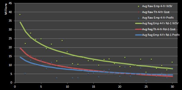
Figure 1: Average Regressed Empirical Four-Year Profit of 1995 — 2012 First-Round Draft Picks

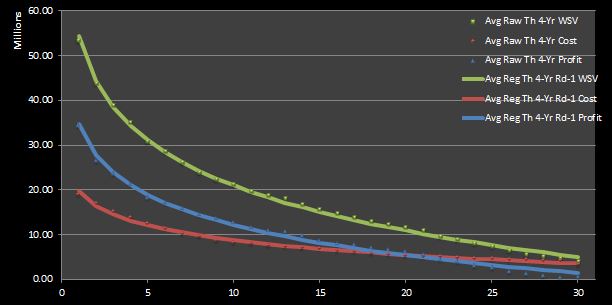
Figure 2: Average Regressed Empirical Four-Year Profit of 1995 — 2012 First-Round Draft Picks

Next, Figure 3 shows the results for IPs calculated with respect to the maximum and minimum data points in four sets of win shares values (WSVs): (1) raw empirical, (2) raw theoretical, (3) regressed empirical, and (4) regressed theoretical.

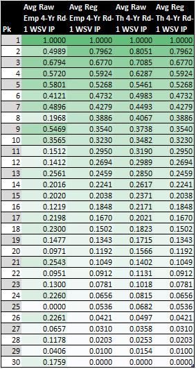
Figure 3: Average Four-Year First-Round WSV IPs

If we use the highest and lowest values in a given range of points as our maximum and minimum points, we can actually calculate 16 different sets of 30 IPs (with one point for each of the 30 first-round picks in each data set).⁵¹ Where does the number 16 come from?

I have four data sets for first-round picks: (1) WS, (2) WSV, (3) cost, and (4) profit. Also, we can permute each data set over two options of two variations: (1) empirical or theoretical data; (2) raw or regressed data. Basically, it comes down to four times two squared. Put even less formally, 16 IP sets: 4 data sets * (2 variations) ^ (2 options)).⁵²

In you work out the math for all 16 IPs, you will find that the IPs for WS and WSV are nearly identical to one another for both the raw empirical and theoretical data. (Intuitively, this makes sense because WSV is just a scaled version of WS, and IPs are simply relative probabilities.) Furthermore, the four regressed forms of empirical and theoretical variations of data are completely coherent (i.e. exactly identical to one another). Thus, there are really only 10 unique sets of IPs. Four of these are shown in Figure 1 (i.e. the raw and regressed empirical and theoretical WS IPs). Not shown are the six other unique sets of IPs: two sets for raw empirical and theoretical WSVs, two sets for raw empirical and theoretical WSVs, and two sets for raw empirical and theoretical profit. (Recall that the regressed forms of these six sets are exactly equivalent to the two sets regressed WSV IPs shown in Figure 3.) So what if I lied when I said there were 16 different IP sets.

5.2.1 Return on Investment (ROI)

Before doing some interesting analysis with our calculated IPs, I want to review some of our data regarding value, cost, and profit in order to better contextualize my upcoming look on market inefficiencies.

If I may go back to using economics terminology for a moment, I can formally prove the notion of diminishing returns that was implied by the profit curves that we saw before.

We can calculate return on investment (ROI), which is just the quotient of the profit and the cost, to verify that higher picks are the most cost-effective. Figure 4 depicts the ROI found using the raw and regressed theoretical four-year profits, as well as the raw theoretical four-year costs.⁵³

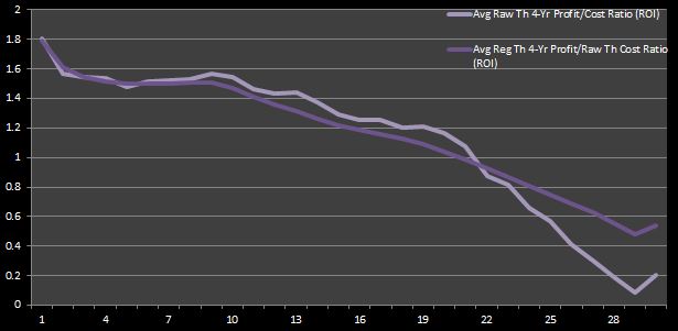
Figure 4: Average Theoretical Four-Year WSV to Cost Ratios (ROI)

The decaying behavior of ROI is not all too surprising, given our prior conclusion that top picks are coveted because top-level talent, which is most commonly acquired through high first-round draft picks, is extremely significant in the NBA, perhaps more so than in any other team sport league. My point is to show that top-picks are the most cost-effective.

5.2.2 Market Inefficiency

So maybe the ROI concept seems like nothing new to you. You’re right, it really isn’t—it’s just a different way of contextualizing what we have already seen. Nevertheless, I thought it was important to introduce it in order to better understand how we can relate the term “market inefficiency” to our discussion.

In particular, I am using the term to distinguish a pick from which the profit exceeds the cost correlated with that pick, relative to the rest of the picks. The key word to recognize here is “relative”. Although ROI proves that the top picks are the most cost-effective, it does so in an absolute sense. That is, it doesn’t really distinguish whether or not the profit produced at a particular draft slot is greater than what is expected by the rookie wage scale.

This is where IPs come back into play—they can be used to identify market inefficiencies. In specific, if I take the difference of the IPs for WSV and the theoretical four-year cost, then I can pinpoint draft slots where player production outperforms that which is dictated by cost. But which of the four sets of WSV IPs should I use?

For the sake of argument, let’s neglect the empirical WSVs for right now. I can argue that the set of raw empirical WSVs  (the data set with the largest standard deviation for each point) are somewhat arbitrary and are biased by the drafting team and chosen player. Consequently, the regressed empirical WSVs are smoothed out too strongly by my linear-log regression to make this data set significant judgement in this nuanced analysis.

That leaves us with the raw and regressed theoretical WSV IPs with which to compare to the theoretical cost IPs. I think that it is difficult to make a convincing judgement call between these two. On one hand, the significance of the raw theoretical WSVs is hindered somewhat by its derivation from empirical values. They are simply a re-ordering onfthe non-linear, non-Guassian distribution of empirical WSV, so they are also somewhat random. On the other hand, the regressed theoretical WSV set may eliminate the effect of reality to too great of an extent.⁵⁴

Why not leave our judgement until we see how each stacks up in tabular and graphical form? Figure 5 shows __both theoretica__l WSV data sets, along with the cost IPs. Because it is somewhat difficult to see where the curves differ the most on their descents, I have also graphed the differentials of the IPs in Figure 6. Also, in case in you were wondering how the empirical WSV points look, Figure 7 is the analogue of Figure 6 with the empirical WSV sets (that I said should be neglected) instead of their theoretical counterparts.

The market inefficiencies can be defined in Figure 5 as the areas along horizontal axis where the cost curve lies above the WSV curve. Likewise, these points of interests are the positive values in Figures 6 and 7.

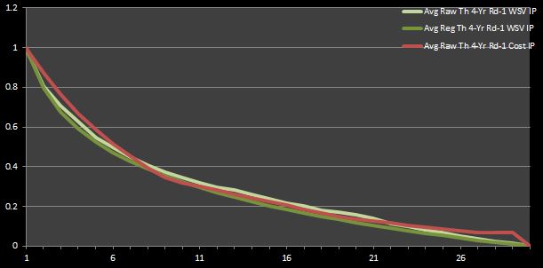
Figure 5: Average Theoretical Four-Year First-Round WSV and Cost IPs

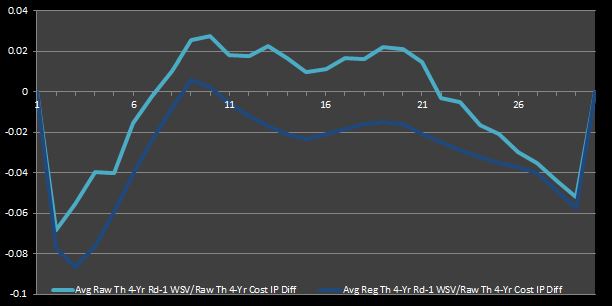
Figure 6: Average Theoretical Four-Year First-Round WSV to Cost IP Differentials

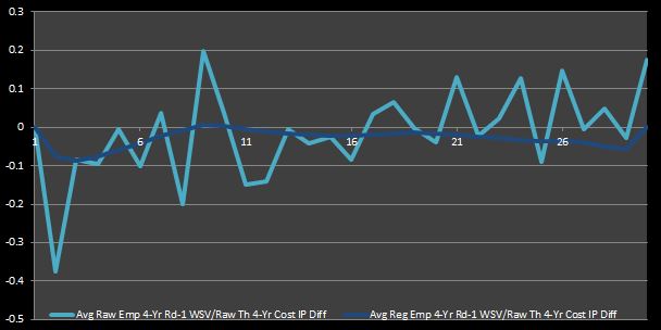
Figure 7: Average Emperical Four-Year First-Round WSV to Cost IP Differentials

I think the inconsistency between the two empirical WSV lines in Figure 7 justifies my prior argument that they should be disregarded for this analysis. On the other hand, it is clear that the raw and regressed curves in Figure 6 behave in the same manner. However, despite their similar behavior, the vertical difference between the lines in Figure 6 can lead to somewhat different conclusions. If the raw values are accepted, then one might deduce that nearly half of the first-round picks (specifically, picks 8 through 21) symbolize market inefficiencies. On the other hand, if the regressed values are taken as a baseline, then one would find that only two first-round picks represent true bargains (specifically, the ninth and tenth picks).

Thus, it is clear how one can deduce different results dependent on which data set is taken as truth. Nevertheless, taking both curves in Figure 6 into account, we can infer that mid-first-round picks are cost-effective relative to early- and late-first-round slots.

5.3 To Be Continued

I believe that this is about as far as I can come in analyzing the value of first-round picks in the NBA draft. With the conclusion that I drew in the preceding section, I have found an answer to the (re-stated) second big question that I asked about NBA draft pick value (“At which draft slots does the expected basketball production outperform the contractual obligation the most?”) in a previous chapter.

As for my third question about pick trade value, I could use my existing IP sets to tackle this topic, but I don’t think I would provide meaningful insight because, in my opinion, the trade values should encompass both first and second round pick.

Thus, I must attempt to model second-round picks and re-calculate IPs in order to give a worthwhile answer to this question. However, I will leave this task for another time.

---

51. As a note to the reader, the next couple of paragraphs discuss nuanced details about the IPs that I can calculate with my existing data sets. So, if you couldn’t care less about these kinds of details, go ahead and skip to the next section.↩

52. As a technical note, I have chosen to shown the IP values for WSVs instead of those for win shares (WS), cost, or profit because they will be used in the upcoming analysis on market inefficiencies.↩

53. I have chosen to use these data sets for the same reasons outlined in detail in the following argument regarding which WSV IPs to use.↩

54. In case you were wondering, I have simply chosen the raw theoretical four-year cost IPs instead of its regressed counterparts because the raw values mirror the actual rookie wage scale.↩