2 What Research Says about NBA Draft Pick Value, Part 2
Having asked and answered the biggest question(s) about the value of NBA draft picks in my last chapter, there are a couple more questions that I sought to have answered (and will attempt to answer myself in my upcoming step-by-step guide to estimating NBA draft pick value.) If you haven’t read that post, you should definitely check it out because I will reference some of the research discussed there in this chapter.
2.1 More Questions
2.1.1 The Third Question
Picking up where I left off, I can articulate two other questions (i.e. “third” and “fourth” questions) that I sought to answer in my earlier review of existing research.13
In considering the meaning of “value” as I did before, I think answers for this question contextualized in terms of either basketball production or monetary cost are equally valid. Some general managers might be fascinated with the superstar potential of a particular prospect and, consequently, would be willing to give up other assets (e.g. experienced players, future picks, etc.) to move up in the draft and pick that talented player. On the other hand, some may be more concerned with cap considerations or trying to “beat the market” by moving into slots that are most “cost-effective”.14
2.1.2 The Fourth (and Final) Question

Finally, the last question that I looked to answer (for now) is “Can tanking be justified?”15
Even though this fourth question does not explicitly include the word “value”, I believe that its answer is still dependent upon the word’s interpretation. In this context, it is probably easiest to interpret its answer on the basis of on-court basketball production, as opposed to off-court monetary cost. In particular, I think a reasonable analysis of the question might compare the chances of a team winning the championship against the likelihood of improving the team with a higher draft pick. In this case, it might be necessary to evaluate “value” on a relative scale because winning a championship is a binary variable (i.e win or no win), whereas the unit of measurement is different for cost (i.e. $ million for rookie contracts) ands for the researcher’s statistic(s) of choice for quantifying basketball production (e.g. an “all-in-one” metric like win shares (WS)).
As you can see from this caveat-filled discussion (as well as the one in my last post) the term “value” is fairly ambiguous. Nevertheless, having defined it in a specific way for each question, I think we can now better contextualize the answers provided by existing research.
2.2 More Answers
2.2.1 The Third Answer
My third question is answered directly in one of the articles I have already reviewed. Arturo Galletti translates his regressed “Net Actual Value” values (which he calls “Modeled Values”) to relative ones for the purpose of constructing a pick trade value chart. This chart is shown below.
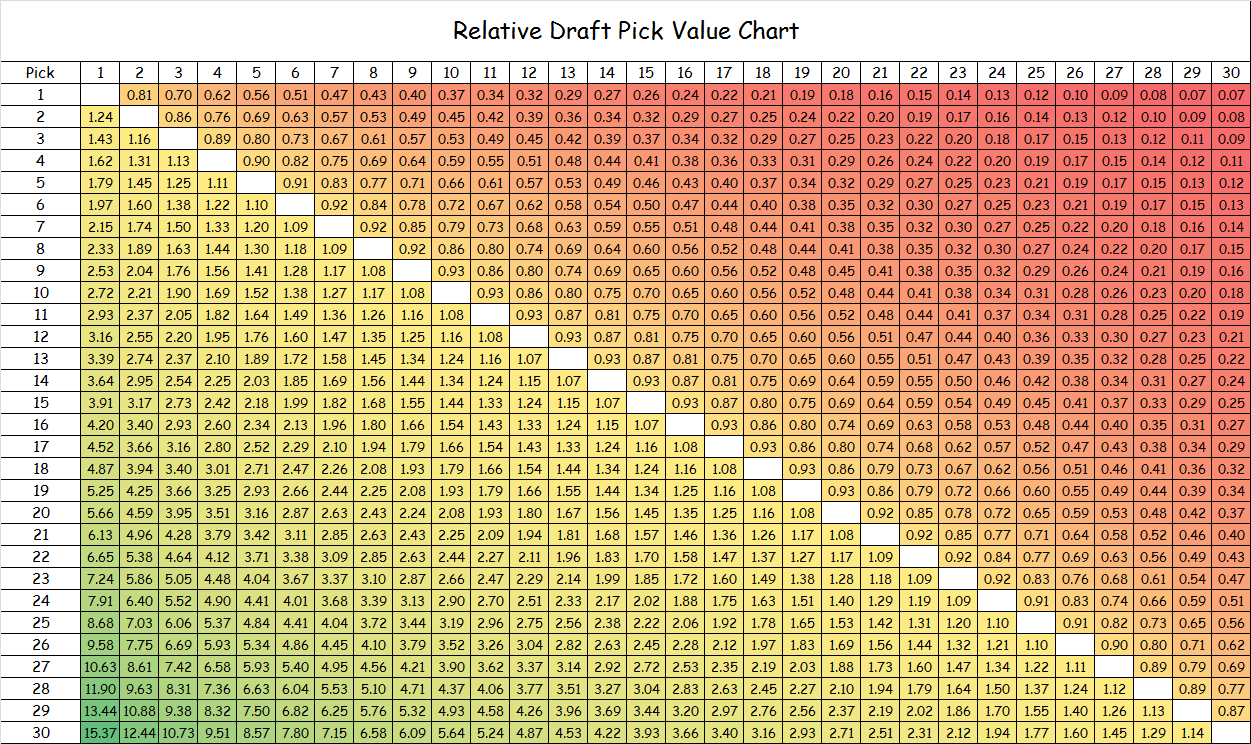
After inspecting Galletti’s regression formula and his numbers for “Modeled Value”, I found that he simply calculates the quotient of the values for any given two picks to come up with their relative trade value. However, I think it is better to use an alternative method that leverages the concept of indifference probability(IP) to calculate relative trade values (as I do in another write-up) where I first scale all the monetary values to a 0-to-1 unit-less basis before taking the quotient of any two values. I believe that my method for calculating relative values using IPs is superior because it does not result in negative values for second-round picks. In particular, if Galletti were to have expanded his chart to include all 60 picks, you would begin to see negative values for picks 38 and below when their values are calculated with respect to the top pick.
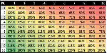
Anyways, the following figure depicts how Galletti’s numbers would look for the top 10 picks using my proposed alternative method using IPs.
Aside from Galletti, Nylon Calculus contributor Nick Restifo provides a trade value chart posted in a recent 2016 article at Fansided. Similar to Saurabh Rane, Restifo uses peak value over replacement player (VORP) values (although he averages over the combined best two-year VORP value rather than simply taking the best single-season value), and, like Michael Lopez, he runs a LOESS regression (although he keeps the raw value of the top pick). Although Restifo’s chart is not normalized like Galletti’s, the value of certain picks relative to one another can be interpreted by finding the absolute difference between the listed values of the picks of interest.16
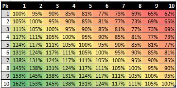
Interestingly, after Restifo’s absolute VORP numbers are normalized to a unit-less 0-to-1 basis using the same alternative method that I used to re-calculate Galletti’s numbers, it turns out that his relative trade value numbers differ relatively dramatically from Galletti’s. The following figure mirrors the same idea shown in the previous figure for Galletti using the calculated relative values for Restifo.
So whose numbers should be taken as truth? As it often seems to be in analytical discussion like this, the answer is “it depends” . We must realize that the two sets of normalized numbers are calculated in a different context—Restifo looks only at_ basketball production, while Galletti discounts on-court value by rookie wage scale cost.
I can make an effort to account for this difference by using Galletti’s regressed “$ Value of Wins” formula estimating the monetary value of wins. Recognizing that this formula—although it is described in units of currency—correlates directly with Galletti’s basketball production “Avg Wins per Pick” data set, I can review how Galletti and Restifo stack up on an equal basis after normalizing these basketball production values with the regression formula that Galletti provides for his “\(alue of Wins [\) million]”.
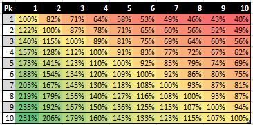
In doing so, I come up with numbers that describe the same idea—basketball production. Having back-tracked Galletti’s numbers to neglect cost, the only difference in the two basketball production estimates is that Galletti’s numbers are based on wins produced (WP), which is fairly similar to win shares (WS), while Restifo’s are based on peak VORP. The following figure shows Galletti’s trade value estimates for the top 10 picks calculated for his basketball production metric.
So, even after accounting for Galletti’s slightly different method of calculating relative values, negating the cost factor incorporated into Galletti’s original numbers, and normalizing the Restifo’s VORP numbers, it still appears that Galletti’s and Restifo’s trade value estimates vary fairly noticeably. (In fact, it appears that their estimates differ even more now!) As I implied before, this difference arises purely from each writer’s choice of basketball-production metric.
Thus, despite my efforts to account for differences in methodology between two researchers, I will leave this discussion at this point. All that is to be said is that the answer to my third question regarding relative trade value depends on your evaluation of the merit of a given advanced metric.
2.2.2 The Fourth (and Final) Answer
Finally, as with my third question, an answer to my fourth question can be found in one of the articles I have already summarized. Rane leverages his estimates for draft pick value contextualized by likelihood of player outcome—All-NBA First-Teamer, All-Star, rotation player, or bust—and normalizes them on a percentage basis to estimate the expected value for a team BEFORE the final lottery spots are determined. The dashed and solid lines in his figure below depict the expected values before and after the teams drafting at each draft slot are finalized. Thus, by looking at Rane’s “prior” and “posterior” estimates, we can simulate the perspective of a team that is bound to miss the playoffs and might reasonably tank in order to improve its lottery odds.
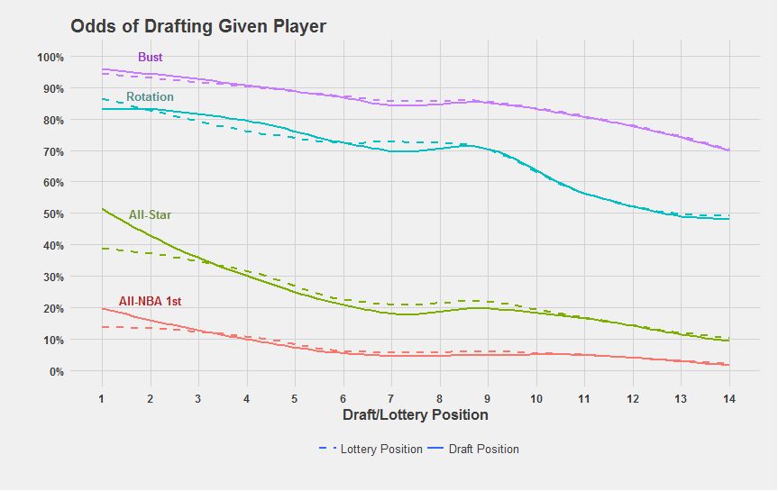
In comparing the two types of lines, Rane notes that tanking when one already has one of the bottom-three or bottom-four win-loss records is not beneficial, as is made evident by the flattening of the dashed curves for the All-NBA First-Teamer and All-Star for the very top draft slots.17 While Rane does not explicitly confirm that the converse is true—that tanking can be beneficial for losing teams that are below average but not egregiously bad—he implies that tanking is not justified for mid-lottery and low-lottery teams either. He notes that the relative indifference in odds of netting an elite player (i.e. All-NBA First-Teamer or All-Star) within the mid-lottery range of picks suggests that these picks aren’t actually as valuable as some pundits have suggested, with respect to producing superstar players. Rather, the linear rise of the rotation and bust lines in the mid-lottery range suggests that higher picks in this range only generate good baseline players (i.e. rotation players or busts) with increased likelihood.18
Rane’s conclusions are backed up by a Journal of Sports Economics study published earlier this year. (This study is concisely summarized by renown American writer Jonah Lehrer on his blog.)19 Published under the lead of Akira Motomura, the research paper concludes that a team’s general management and other intangible infrastructural influences (i.e. “team culture”) has a stronger influence on the success of a team than do the draft slot it earns and the players that they draft. In specific, Motomura et. al. find that picks 1 through 3 tend to have a relatively neutral impact on the near-future win-loss records of their respective teams, that picks 4 through 10 actually have a negative impact over the following years20
A number of factors can explain the conclusion that tanking lacks merit. For one, it is understandable that even the most talented rookies cannot make a huge impact and turn franchises around immediately because they tend to make many more mistakes than their veteran peers, who can make up for any age-induced talent diminishment with their experience and knowledge of the game’s ins-and-outs at the professional level. Veterans tend to garner more respect from referees than younger players, understand the tendencies of opponents after having played them numerous times, and know how to pace themselves in a manner such that they don’t wear down by end of the regular season. Even after young players move on from their rookie seasons, they often don’t mature and reach their full potential for another couple of years.
Aside from the experience advantage that discounts the effect of young players, there is also the fact that picking players in the draft is an inexact science. Teams at the top of the draft often pick players that turn out to be busts. Although tanking can increase the probability of earning a high draft slot, the expected value of a pick is just that—an expectation. There is no guarantee that teams will select the best player for them. As Motomura et. al. argue, drafting players and player development are skills that derive from the foresight and teaching capabilities of the team’s management. Thus, a draft pick’s expected value is heavily influenced by the team that is selecting at that slot, which is not reflected in any publicly available draft pick value model of which I am aware.21
While the research of Rane and Motomura et. al. suggest that tanking is not justified, Arturo Gutierrez finds in his research article The NBA Lottery and Game Theory that there are cases that tanking can be the “correct strategy”. For his analysis, Gutierrez first formulates an estimate of draft pick value by running a polynomial regression over the career WS earned by players drafted by teams ordered by win-loss record.22 Then, he formulates an estimate for the likelihood of a team winning the championship by running a separate regression over the historical results of teams ranked by playoff seed, Next, he compares these regressed curves on a graph over a dependent axis with numbers counting from 1 to 30 in order to represent teams ordered by best win-loss record for any arbitrary season. Finally, after accounting for what he calls the “time value” of winning a championship (such that the values of his regressed curve for championship likelihood are boosted because chances of winning in the near future are added to the single-year values), Gutierrez outputs a graph that indicates that any team worse than the sixth-best team should purposely try to lose.23
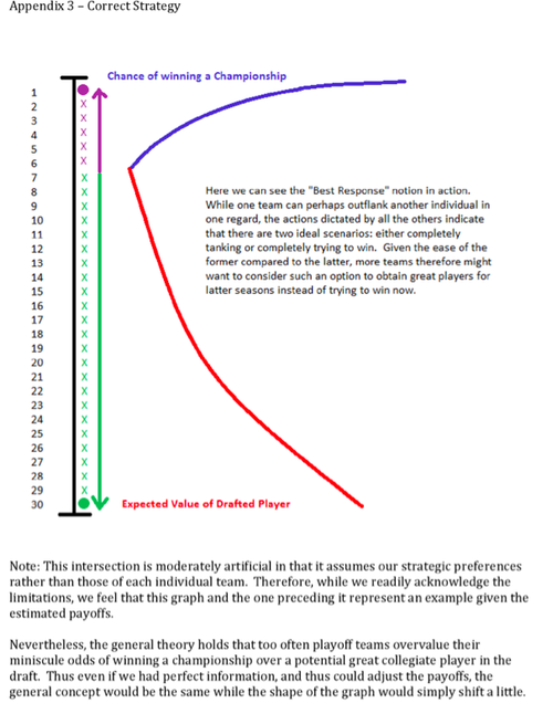
I think that Gutierrez’s perspective on this matter suffers somewhat from its failure to consider mixed strategies and their equilibria. He considers only the pure strategies of expending all effort to be the best team or to be the worst team.24 Nevertheless, Gutierrez admits that there are limitations to his approach. He notes that the “best response” for a given team is dependent on its specific situation, including variable such as the team’s win-loss record and its perception of whether or not other teams are tanking. Thus, even though Gutierrez’s analysis offers some validity to tanking, I don’t think his evidence is sufficiently strong to override the case made by the research of Rane and Motomura et. al.
2.3 Final Thoughts
In my first write-up I took look at the value of draft picks in terms of basketball production and contractual costs after reviewing the methodologies and conclusions of other researchers. There, I found that the answers were fairly the same across all researchers. Moreover, I reviewed only one person (Aaron Barzilai) who really evaluated the cost-effectiveness of picks, a topic which I also plan to explore.
Now, having reviewed what research has to say about the related topics of pick trade value and tanking and having coming to some non-universal answers, I plan to expand my investigation to include these subjects as well.
Actually, to be truthful, I only postulated these questions while looking for answers to my previous two questions. The third question can be simply stated as “What is the relative trade value of picks?”↩
I mentioned the term “cost-effective” in my previous chapter without formally defining it. In reality, economics terms such as “cost-effective”, “beating the market”, and “return on investment” should be formally defined in an NBA context by the person conducting the cost analysis. In any matter, I think that the reader can probably correctly infer the author’s intended meaning if the author neglects to define such terms. Thus, I am interested in trying to come up with the answers to the third question from both kinds of “value” perspectives—purely basketball production and purely monetary cost. In particular, I would say that the monetary interpretation is interesting for identifying general managers who have tried to “outsmart” their colleagues.↩
The term “tanking” refers to a team that intentionally loses to try to improve its odds of winning the NBA lottery. The 14 teams that miss the playoffs are entered into a lottery that determines draft order. The teams with the worst records have the best chances of winning a higher draft slot. More detail about the lottery can be found at the satirical NBA Tankathon website.↩
As an aside, one should realize that, even if the values of two lower picks is equal to that of a single higher one, one might reasonably prefer the higher upside presented by the higher draft pick, while someone else might prefer the “diversification” of having two prospects as opposed to one.↩
On the other hand, the final expected value of lottery picks between 5 and 14 generally is equal to (or greater than) before the finalized allocation of draft picks to teams.↩
On a related note, these trends reaffirm the raw conclusion that we made about the generalized draft pick value question—that basketball production drops off as pick number increases—and give a partial answer to my restated second question from before (“At which draft slots does the expected basketball production outperform the contractual obligation the most?”) Using Rane’s illustrations, we can deduce that, in terms of pure basketball production, the value of mid-lottery and low-lottery picks are highly unlikely to generate elite players. Of course, the conclusions of others who have evaluated draft slots in terms of pure basketball production also implies the same principle, but Rane’s illustrations and rhetoric make this notion definitive.↩
I am thankful to Lehrer for his review of the study because I do not actually have access to the study.↩
Motomura et. al. find that these picks correlate to 6 to 9 more losses three years after the draft year, and that, more generally, all picks in the lottery range (and extending to pick 17) are associated with negative (or negligible at best) team performance. These numbers clearly suggest that tanking is not exactly the best strategy for teams looking to improve.↩
Accounting for how team factors correlate with the value extracted from draft picks would be a very difficult task that would require lots of probabilistic assumptions.↩
In contrast to the methods used by the researchers I discussed in my last chapter, he does not directly relate his choice of basketball production metric (in this case, WS) with draft slot; instead, he factors in the probabilistic relationship of lottery odds with team win loss-record to relate basketball production to teams ranked by record. Also, he uses a polynomial regression rather than a linear-log regression or a LOESS.↩
Without accounting for “time value”, then the intersection point manifests at the third-best team. This graph is shown in the figure below.↩
This perspective is like a manifestation of the idea that I described at the beginning of this chapter—evaluate tanking by comparing draft pick value and championship likelihood from a stict binary point of view.↩